Inverted Double Pendulum
Purpose
The purpose of this example is to introduce students to the interface of Amesim and how to navigate through the software to build a simple example using Amesim’s Planar mechanical library.
Learning Outcome
After following this example, the students will be able to navigate through Amesim and its modes comfortably and will also become familiar with the Planar mechanical library.
Introduction to the problem
Inverted double pendulum is a simple and classic example in the rigid body dynamics field. The system consists of two rigid bodies connected via a pivot junction. One node of one of the bodies is connected to a fixed pivot junction while one end of the other body is a free end. After releasing the system from an initial position, the two bodies move about their respective pivots under the influence of gravitational force.
1. Sketch Mode
Whenever we fire up Amesim, we start off in the Sketch mode by default.
Now, from the Library tree on the right side of your screen, find and double-click on the ‘Planar Mechanical’ library.

Figure 2: Planar Mechanical Library
Then, the Planar Mechanical library will open up and you will be able to see all of its components.

Figure 3: Components of the planar mechanical library
To know what each component is, hover your mouse cursor over the component for a couple of seconds

Figure 4: Revealing the name of any component; Pivot junction
And to know more about any component, right-click on the component and click on ‘Help’

Figure 5: Using the 'Help' option to know more about each component
Now, we proceed to sketch our model. To do this, we need bring all the necessary components to our sketch area. We can do this in two ways:
- Drag and drop
- Click on the component once, move your cursor onto the sketch area and place it by clicking again.
You will see a sketch similar to the following image. The numbers on the either side of the component block are its ports. More about ports later.

Figure 6: Adding components to the sketch
Now, we proceed to sketch our model. To do this, we need bring all the necessary components to our sketch area. We can do this in two ways:
- Drag and drop
- Click on the component once, move your cursor onto the sketch area and place it by clicking again.
You will see a sketch similar to the following image. The numbers on the either side of the component block are its ports. More about ports later.

Figure 7: Components required to complete this example
After you complete importing all the required components to your sketch it should look like this:
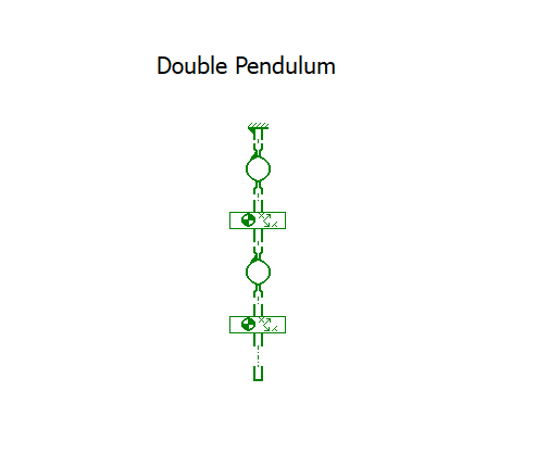
Figure 8: All the components in the sketch before making the connections
Before connecting all our components, which ports of each component needs to be connected to another component. So, it is always a good convention to make sure that the output port number is greater than that of the input. And because the end restraint is the only fixed component in the sketch, we can start from there.
So, we want the output of the end restraint to be connected to the input of the pivot junction. We can always rotate a component by using the Ctrl + R shortcut. Then, arrange your components such that input port number is 1.
Now, we need to make the connections. To do this click near the port of one component to see your cursor turn to a black plus symbol. Now you should be able to see a green dot-dashed line following your cursor. Move your cursor close to the port of the component to which you want to connect your first component until you see a green square appear. Then, click again. Now, both the components are connected together. Follow the same procedure to connect all the components.

Figure 9: Port numbers of a component and making connections
At the end of it, your sketch should look like this:

Figure 10: Sketch after completing the connections
You can always drag any component to rearrange your sketch. Note that you cannot rotate or flip (Ctrl + M) your components after making the connections.

Figure 11: Rearranging your components
Now, our sketch is ready. Using Ctrl+S, save the file to a local drive and make sure that the file name does not have any spaces, and it should also not start with a number.
Before we windup our sketch, we need two more supplementary components which are not a part of our problem, but are necessary for our simulation. Those are the assembly component from the Planar mechanical library and the gravity icon from the Mechanical library.

Figure 12: Auxiliary components required

Figure 12: Auxiliary components required
2. Sub-model Mode/ Step2
After completing the assembly of our components, the next step in building our model is the Sub-model mode.

After we switch to this mode, we will see that some components get highlighted. This means that those components have multiple sub-models from which we can select one. By selecting different sub-models, we are choosing a more complex mathematical representation of the same component.

Figure 13: Highlighted components in sub-model mode
We can see the list of sub-models of a particular component by double-clicking on the highlighted component.

Figure 14: List of sub-models available for any component
Here, we can see that the pivot junction component has two sub-models. Generally, the sub-models are listed in the order of increasing complexity i.e. PLMPIV01 is more complex than PLMPIV00.
If we just want all the simplest mathematical models for all the components which have multiple sub-models, we can do so by directly selecting the Premier Sub-model option.

3. Parametric Mode/ Step3
Now that we have defined how each component is mathematically represented, the next step is to define the parameters of each component. We do this in the Parametric mode.

Parameters of every component can be seen on the right hand side of the screen, after clicking on the component of interest. In the following image we can see the parameters of the end restraint component.
For the problem of interest, we do not change any of these parameters as we want the end restraint to serve as the origin, relative to which we will define the components connected to it.

Figure 15: Parameters of the end restraint
Next, we set the parameters for the pivot junction. Ideally, a pivot should not have any stiffness or damping associated with it. So, to make things simple when we try to validate our simulations with hand-written solutions, it is better to set these parameters to 0. Make sure to do this for both the pivot junctions.

Figure 16: Parameters of the pivot junction
Then, we have to define the parameters of the PLM body-1. Whenever dealing with most of the components in the Planar mechanical library, it is important to visualize these components in a coordinate plane, and the parameters that we set will define their position in that coordinate plane.
Let the following be the parameters for the two bodies in our problem
Parameter |
Magnitude |
Length of body-1 |
1 m |
Mass of body-1 |
1 kg |
Orientation of body-1 |
00 |
Length of body-2 |
1 m |
Mass of body-2 |
1.5 kg |
Orientation of body-2 |
300 |
Because the length of our Body-1 is 1 m, the parameter ‘x position at port 2’ should be set to 1 m. This is because port 1 is attached to the pivot which in turn is attached to the end restraint (our origin), so naturally port 2 should be the length of the body. As a consequence, the center of gravity parameter ‘G: initial relative x position’ should be 0.5, assuming that our body is uniformly distributed.
Following the formula, , for Moment of inertia of a rod, we can set the parameter ‘moment of inertia around Gz axis’
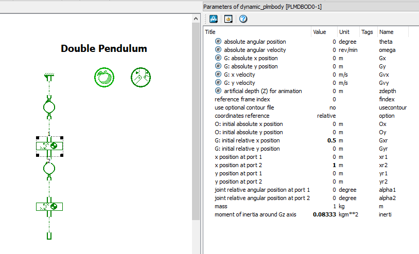
Figure 17: Parameters of the PLM body
Now, we need to follow the same procedure to set the parameters for our Body-2. Before we do that, we need to look at another parameter: coordinates reference. If this parameter is set to relative, then it means that the coordinates for this particular body need not be calculated from the origin. In this case, port 1, becomes the new origin and so the parameters of the body can be set in the same manner as we did for Body-1. If we have the ‘coordinates reference’ as absolute, the x position at port 1 will be 1 m and x position at port 2 will be 2 m.

Figure 18: Coordinates reference parameter of PLM body
4. Simulation Mode/ Step4
At this stage, we have built our sketch, chose the mathematical representation of the components, and finally defined the parameters of all the components. Next step is to run the simulation.

As soon as we click on the simulation mode button, Amesim compiles the model that we have built and creates a simulation program
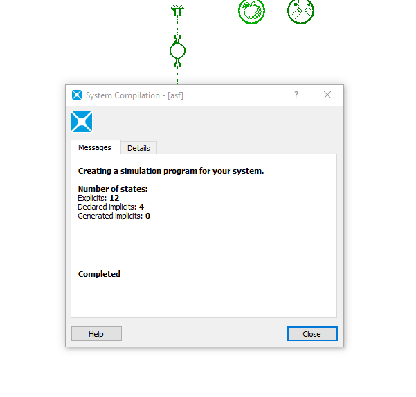
Figure 19: System compilation window
If we have built our model correctly, then we will see the ‘Completed’ message after system compilation.

We can change the parameters of our simulation, by clicking on the ‘Run parameters’ button

Figure 20: Run parameters window
For the example in consideration, we need not change any of these parameters.
Then, we click on the ‘Start simulation’ button to run the model.
If we haven’t made any mistakes in building our model, then the simulation will run to 100% without any errors.

Figure 21: Successful simulation
5. Visualizing Results
Now that we have successfully run our simulation without any errors, it is time to visualize and analyze the parameters of interest. The outputs/variables of any component can be seen on the right, bottom corner of the screen.

Figure 22: Variables/Outputs of the PLM body-2
Suppose we want to visualize how the angular position of Body-2 has changed over time, we need to plot it.
In Amesim, plotting any result is as easy as a drag and drop. Click on Body-2 to display its variables. Now, click on ‘absolute angular position’ and drag it on to the sketch and release the mouse button.
Now, we will be able to see a plot of ‘absolute angular position [degree] vs Time [s]’

Figure 23: Absolute angular position of PLM body-2 vs Time
You can follow the same procedure to plot any variable of any component in your model.
There is one feature in Amesim which is specific to the Planar mechanical library: PLM-Assembly. In any other library, we can visualize the functioning of our system by building a 3d representation using Amesim’s Animation feature, but the PLM-Assembly block automatically builds the animation using the parameters that we set.
You can open the animation by double-clicking on the PLM-Assembly component.

Figure 24: Interface of the PLM assembly animation window
Here, you can see that all the components that we had used to build our model have been represented in the animation.
You can click on the play button on top of the animation window to visualize the functioning of our double pendulum system.
Example By: Sai Krishna Sumanth Nakka